Fluorescence lifetime imaging with LINCam, analysed with PhasorPy, the open-source phasor library: the 284 million photons of a Convallaria majalis section separate into three lifetime populations, and every pixel into a share of two lifetimes, without a single fit.

The phasor approach turns the fluorescence decay of each pixel into two numbers, the cosine and the sine coefficient of its Fourier series at one frequency. A decay with a single lifetime lands on a semicircle; a mixture of lifetimes lands inside it, on the line between its components, at a place set by their share of the photons. Nothing is fitted and nothing is assumed about how many lifetimes there are: populations show as clusters on the plot, and a cluster picked there points back to its pixels in the image.

PhasorPy is an open-source Python library for the analysis of luminescence lifetime and hyperspectral images using the phasor approach. It reads the files of many microscopes itself; for LINCam, the photonscore Python package reads the .photons file and histograms the photons, and PhasorPy takes over from the histogram.

LINCam records the position and the arrival time of every photon, so the histogram is made after the measurement, at any pixel size and any time binning. Its 4096 channels of 12.3 ps span 50.4 ns and hold the whole decay: the histogram is one period of a periodic signal, and every harmonic of 19.8 MHz gives a phasor of its own.

Results

The recording holds 284,223,008 photons in 1371 s, histogrammed at 512 × 512 pixels and 256 time bins. The 74,426 pixels with 300 photons or more hold 97 % of them; their phasors were median-filtered. At the third harmonic, 59.5 MHz, lifetimes of 0.5 to 3 ns spread over most of the semicircle, and the phasors of the section form an elongated cloud inside it (Figure 1, top right).

A Gaussian mixture finds three populations on the plot. Mapped back to the image, they are the anatomy of the section: the S-shaped group of cells in its centre, the bright band at its edge, and the dimmer tissue between them, with phase lifetimes of 1.93, 1.52 and 0.99 ns and modulation lifetimes of 2.68, 2.22 and 1.78 ns. Phase and modulation lifetime differ in every population: no pixel decays with a single lifetime.

The long axis of the cloud meets the semicircle at 0.64 and 2.92 ns. Read as mixtures of these two lifetimes, the pixels hold a quarter of their photons in the shorter one in the central cells, two fifths in the band and two thirds in the dim tissue (Figure 1, bottom right). The cloud is wider than a line, so more than two lifetimes are at work, and the share summarises a pixel rather than fits it. A fit of the same recording with four lifetimes is application note 3.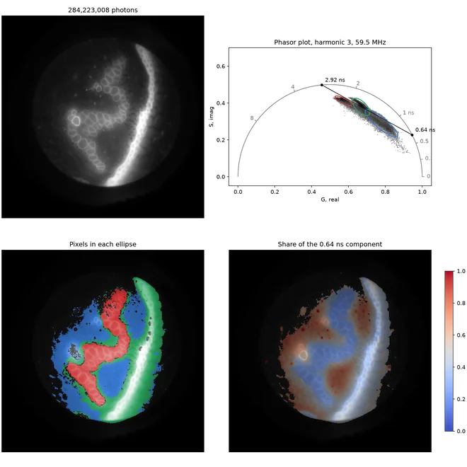

Calibration

Uncalibrated phasors are rotated by where the laser pulse falls in the TAC range, 10.5 ns here, and shrunk by the width of the instrument response. PhasorPy calibrates against a reference of known lifetime, and for LINCam the instrument response itself will do: some 80 ps wide, far narrower than a period at these frequencies, its phasor is a point on the unit circle at the phase of time zero, a reference of lifetime 0. Time zero is where the decay of all photons climbs fastest, 10.523 ns in this recording. On simulated photons this lands within 3 ps of the true response, and single exponentials of 0.5, 2 and 4 ns come out within 0.0005 of their places on the semicircle.

The whole analysis takes some 15 seconds on a laptop: 11 s to read and histogram the file, streamed in chunks so that the memory in use stays near 2 GB, and a fraction of a second for the phasors of a quarter of a million pixels.

Sample

A section of Convallaria majalis (lily of the valley) rhizome, the usual test slide for fluorescence lifetime imaging, recorded by André Weber with a LINCam on a Nikon Eclipse Ti microscope.

Data and code

The script phasor.py and the notebook phasor.ipynb, with a README on how to install and run them, are on GitHub. They need the photonscore Python package from our downloads page and PhasorPy. The phasors are saved as an OME-TIFF that PhasorPy reads back.

PhasorPy is cited as doi:10.5281/zenodo.13862586.